Case Study: Outliers and Bayesian Integrals
In this case study, we analyze a fit with outliers in the data that distort the least-squares solution. We show one approach to dealing with the outliers that requires using Bayesian integrals in place of least-squares fitting, to fit the data while also modeling the outliers.
This case study is adapted from an example by Jake Vanderplas
on his Python blog.
It is also discussed in the documentation for the vegas module.
The Problem
We want to extrapolate a set of data values y to x=0 fitting
a linear fit function (fitfcn(x,p)) to the data:
import numpy as np

import gvar as gv
import lsqfit

def main():
    # least-squares fit to the data
    x = np.array([
        0.2, 0.4, 0.6, 0.8, 1.,
        1.2, 1.4, 1.6, 1.8, 2.,
        2.2, 2.4, 2.6, 2.8, 3.,
        3.2, 3.4, 3.6, 3.8
        ])
    y = gv.gvar([
        '0.38(20)', '2.89(20)', '0.85(20)', '0.59(20)', '2.88(20)',
        '1.44(20)', '0.73(20)', '1.23(20)', '1.68(20)', '1.36(20)',
        '1.51(20)', '1.73(20)', '2.16(20)', '1.85(20)', '2.00(20)',
        '2.11(20)', '2.75(20)', '0.86(20)', '2.73(20)'
        ])
    fit = lsqfit.nonlinear_fit(data=(x, y), prior=make_prior(), fcn=fitfcn)
    print(fit)

def fitfcn(x, p):
    c = p['c']
    return c[0] + c[1] * x

def make_prior():
    prior = gv.BufferDict(c=gv.gvar(['0(5)', '0(5)']))
    return prior


if __name__ == '__main__':
    main()
The fit is not good, with a chi**2 per degree of freedom that is
much larger than one, despite rather broad priors for the intercept and
slope:
Least Squares Fit:
  chi2/dof [dof] = 13 [19]    Q = 1.2e-40    logGBF = -117.45

Parameters:
            c 0   1.149 (95)     [    0 ± 5.0 ]
              1   0.261 (42)     [    0 ± 5.0 ]

Settings:
  svdcut/n = 1e-12/0    tol = (1e-08*,1e-10,1e-10)    (itns/time = 5/0.1s)
The problem is evident if we plot the data:
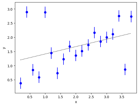
At least three of the data points are outliers: they disagree with other
nearby points by several standard deviations. These outliers have a big
impact on the fit (dashed line). In particular they pull the x=0 intercept (fit.p['c'][0])
up above one, while the rest of the data suggest an intercept of 0.5
or less.
A Solution
There are many ad hoc prescriptions for handling outliers. In the best
of situations one would have an explanation for the outliers and seek
to model them accordingly. For example,
we might know that some fraction w of the time our detector
malfunctions, resulting in much larger measurement errors than usual.
This model can be represented by a more complicated probability
density function (PDF) for the data that consists of a linear combination
of the normal PDF with another PDF that is similar but with much larger
errors. The relative weights assigned to these two terms would be 1-w
and w, respectively.
A modified data prior of this sort is incompatible with the least-squares
code in lsqfit. Here we will incorporate it by replacing the
least-squares analysis with a Bayesian integral, where the normal PDF is
replaced by a modified PDF of the sort described above.
The complete code for this analysis is
as follows:
import numpy as np
import gvar as gv
import lsqfit
import vegas

def main():
    ### 1) least-squares fit to the data
    x = np.array([
        0.2, 0.4, 0.6, 0.8, 1.,
        1.2, 1.4, 1.6, 1.8, 2.,
        2.2, 2.4, 2.6, 2.8, 3.,
        3.2, 3.4, 3.6, 3.8
        ])
    y = gv.gvar([
        '0.38(20)', '2.89(20)', '0.85(20)', '0.59(20)', '2.88(20)',
        '1.44(20)', '0.73(20)', '1.23(20)', '1.68(20)', '1.36(20)',
        '1.51(20)', '1.73(20)', '2.16(20)', '1.85(20)', '2.00(20)',
        '2.11(20)', '2.75(20)', '0.86(20)', '2.73(20)'
        ])
    prior = make_prior()

    print(20 * '-', 'nonlinear_fit')
    fit = lsqfit.nonlinear_fit(data=(x, y), prior=prior, fcn=fitfcn)
    print(fit)

    ### 2) Bayesian integrals with modified PDF
    print(20 * '-', 'Bayesian integral fit')
    modpdf = ModifiedPDF(data=(x, y), fitfcn=fitfcn, prior=prior)

    # integrator for expectation values with modified PDF
    modpdf_ev = vegas.PDFIntegrator(param=fit.p, pdf=modpdf)

    # adapt integrator to pdf
    modpdf_ev(neval=4000, nitn=10)

    # calculate means and covariances of g(p)
    @vegas.rbatchintegrand
    def f(p):
        return {k:p[k] for k in ['c', 'b', 'w']}
    s = modpdf_ev.stats(f)

    # print out results
    print(s.summary())
    print('c =', s['c'])
    print('corr(c) =', str(gv.evalcorr(s['c'])).replace('\n', '\n' + 10*' '), '\n')
    print('b =', s['b'])
    print('w =', s['w'], '\n')
    print('logBF =', np.log(s.pdfnorm))

def fitfcn(x, p):
    c = p['c']
    return c[0] + c[1] * x

def make_prior():
    prior = gv.BufferDict(c=gv.gvar(['0(5)', '0(5)']))
    prior['gb(b)'] = gv.BufferDict.uniform('gb', 5., 20.)
    prior['gw(w)'] = gv.BufferDict.uniform('gw', 0., 1.)
    return prior

@vegas.rbatchintegrand
class ModifiedPDF:
    """ Modified PDF to account for measurement failure. """
    def __init__(self, data, fitfcn, prior):
        x, y = data
        self.fitfcn = fitfcn
        self.prior_pdf = gv.PDF(prior, mode='rbatch')
        # add rbatch index
        self.x = x[:, None]
        self.ymean = gv.mean(y)[:, None]
        self.yvar = gv.var(y)[:, None]

    def __call__(self, p):
        w = p['w']
        b = p['b']

        # modified PDF for data
        fxp = self.fitfcn(self.x, p)
        chi2 = (self.ymean - fxp) ** 2 / self.yvar
        norm = np.sqrt(2 * np.pi * self.yvar)
        y_pdf = np.exp(-chi2 / 2) / norm
        yb_pdf = np.exp(-chi2 / (2 * b**2)) / (b * norm)
        # product over probabilities for each y[i]
        data_pdf = np.prod((1 - w) * y_pdf + w * yb_pdf, axis=0)

        # multiply by prior PDF
        return data_pdf * self.prior_pdf(p)

if __name__ == '__main__':
    main()
Here class ModifiedPDF implements the modified PDF. As usual the PDF for
the parameters (in __call__) is the product of a PDF for the data times a
PDF for the priors. The data PDF is the product of the PDFs for each data point,
but the latter PDFs are more complicated than usual as
they consists of two Gaussian distributions: one with the
nominal data errors (y_pdf), and the other with errors that are b times
times larger (yb_pdf). The prior’s PDF is Gaussian and here is implemented
use gvar.PDF. Parameter w determines the relative weight of each data PDF.
ModifiedPDF is designed to handle integration points in batches
(@vegas.rbatchintegrand): the parameters p[k] have an extra
index on the right labeling the integration point (e.g., p['b'][i]
and p['c'][d,i] where ``i is the batch index).
This makes for substantially faster integrals.
The Bayesian integrals are estimated using vegas.PDFIntegrator
modpdf_ev, which is created from the least-squares fit output (fit).
It is used to evaluate expectation values of arbitrary functions of the
fit variables with respect to a modified PDF modpdf (an instance
of class ModifiedPDF).
We have modified make_prior() to introduce w and b
as new fit
parameters. The prior for w is uniformly distributed
across the interval from 0 to 1, while b’s prior is
uniformly distributed between 5 and 20. Parameters w and b play
no role in the initial least-squares fit. (The uniform distributions are implemented
by introducing functions gw(w) and gb(b) that map them onto Gaussian
distributions 0 ± 1. The integration parameters in the
Bayesian integrals are gw(w) and gb(b) but the BufferDict dictionary
makes the corresponding values of w and b available automatically.)
We first call modpdf_ev with no function, to allow the integrator to adapt
to the modified PDF. We then use modpdf_ev.stats(f) to calculate the
means, standard deviations, and covariances of the fit parameters in the
dictionary returned by
function f(p). The output dictionary s
contains expectation values (gvar.GVars) for the corresponding entries in f(p).
The results from this code are as follows:
-------------------- nonlinear_fit
Least Squares Fit:
  chi2/dof [dof] = 13 [19]    Q = 1.2e-40    logGBF = -117.45

Parameters:
            c 0          1.149 (95)        [    0 ± 5.0 ]
              1          0.261 (42)        [    0 ± 5.0 ]
          gb(b)   8.33405e-15 ± 1.0        [    0 ± 1.0 ]
          gw(w)   8.33405e-15 ± 1.0        [    0 ± 1.0 ]
---------------------------------------------------------
              b          12.5 (6.0)        [ 12.5 (6.0) ]
              w           0.50 (40)        [  0.50 (40) ]

Settings:
  svdcut/n = 1e-12/0    tol = (1e-08*,1e-10,1e-10)    (itns/time = 5/0.1s)

-------------------- Bayesian integral fit
itn   integral        average         chi2/dof        Q
-------------------------------------------------------
  1   4.599(31)e-11   4.599(31)e-11       0.00     1.00
  2   4.542(32)e-11   4.571(23)e-11       0.80     0.68
  3   4.447(33)e-11   4.530(19)e-11       1.49     0.04
  4   4.518(32)e-11   4.527(16)e-11       1.38     0.04
  5   4.515(32)e-11   4.524(14)e-11       1.21     0.12
  6   4.561(34)e-11   4.530(13)e-11       1.13     0.21
  7   4.571(32)e-11   4.536(12)e-11       1.04     0.37
  8   4.518(37)e-11   4.534(12)e-11       0.98     0.55
  9   4.543(33)e-11   4.535(11)e-11       0.95     0.64
 10   4.533(32)e-11   4.535(10)e-11       0.94     0.67

c = [0.29(14) 0.619(60)]
corr(c) = [[ 1.         -0.90215491]
           [-0.90215491  1.        ]]

b = 10.6(3.6)
w = 0.27(12)

logBF = -23.8167(23)
The table after the fit shows results for the normalization of the
modified PDF from each of nitn=10 iterations of the vegas
algorithm used to estimate the integrals. The logarithm of the normalization
(logBF) is -23.8, which is much larger than the value -117.5 of logGBF
from the least-squares fit. This means that the data much prefer the
modified PDF (by a factor of exp(-23.8 + 117.4) or about 1040).
The new fit parameters are much more reasonable. In particular the intercept is 0.29(14) rather than the 1.15(10) from the least-squares fit. This is much better suited to the data (see the dashed line in red, with the red band showing the 1-sigma region about the best fit):
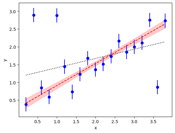
Note, from the correlation matrix, that the intercept and slope are
anti-correlated, as one might guess for this fit.
The analysis also gives us an estimate for the failure rate w=0.27(12)
of our detectors (they fail about a quarter of the time) and the
extent b=11(4) of the failure (errors are about 11 times larger).
A Variation
A slightly different model for the failure that
leads to outliers assigns a different w to each data point.
It is easily implemented here by changing the prior
so that w is an array:
def make_prior():
    prior = gv.BufferDict(c=gv.gvar(['0(5)', '0(5)']))
    prior['gb(b)'] = gv.BufferDict.uniform('gb', 5., 20.)
    prior['gw(w)'] = gv.BufferDict.uniform('gw', 0., 1., shape=19)
    return prior
The Bayesian integral then has 22 parameters, rather than the 4 parameters before. The code still takes only a few seconds to run (on a 2020 laptop).
The final results are quite similar to the other model:
c = [0.31(17) 0.608(71)]
corr(c) = [[ 1.         -0.90853691]
           [-0.90853691  1.        ]]

b = 8.8(3.1)
w = [0.37(27) 0.66(23) 0.39(27) 0.41(27) 0.66(24) 0.50(28) 0.54(29) 0.36(26)
 0.43(29) 0.40(26) 0.40(27) 0.35(26) 0.42(28) 0.38(27) 0.39(26) 0.39(27)
 0.48(29) 0.68(23) 0.36(27)]

logBF = -24.379(41)
Note that the logarithm of the Bayes Factor logBF is slightly lower for
this model than before. It is also less accurately determined (18x), because
22-parameter integrals are considerably more difficult than 4-parameter
integrals. More precision can be obtained by increasing neval, but
the current precision is more than adequate.
Only three of the w[i] values listed in the output are more than two
standard deviations away from zero. Not surprisingly, these correspond to
the unambiguous outliers.
The outliers in this case are pretty obvious; one is tempted to simply drop
them. It is clearly better, however, to understand why they have occurred and
to quantify the effect if possible, as above. Dropping outliers would be much
more difficult if they were, say, three times closer to the rest of the data.
The least-squares fit would still be poor (chi**2 per degree of freedom of
3) and its intercept a bit too high (0.6(1)). Using the modified PDF, on the
other hand, would give results very similar to what we obtained above: for
example, the intercept would be 0.35(17).