Case Study: Fitting a Spline
This study shows how to fit noisy data when the underlying functional form is unknown. The function is modeled with a spline.
The Problem
Our goal is to determine a function f(m) from data for a
different function F(m,a) where
F(m,a) = f(m) + sum_n c_n * (a*m) ** (2*n)
and the sum is over positive integers (n=1,2,3...).
So f(m) = F(m,a=0) is the desired output. We have
three sets of data, each with a different value of a
and a variety of m values:
set  1/a  a*m    F(m,a)
-----------------------
  A 10.0  0.1  0.41(10)
          0.3  0.89(10)
          0.5  1.04(10)
          0.7  1.21(10)
          0.9  1.63(10)
-----------------------
  B  5.0  0.3  0.68(10)
          0.5  0.94(10)
          0.7  1.17(10)
          0.9  1.57(10)
-----------------------
  C  2.5  0.5  0.70(10)
          0.7  1.00(10)
          0.9  1.47(10)
-----------------------
There are statistical correlations between the data values,
so we have dumped the data (using gvar.dump(data, 'spline.p'))
into a file called 'spline.p' that can be read by
the fit code.
We do not know the functional form of f(m), so we
parameterize it using a cubic spline, where the function
is described by specifying its values at specific points
called knots. The spline approximates the function between
each adjacent pair of knots with a cubic polynomial tailored
to that interval. The polynomials are stitched together
at the knots to keep
the function smooth from one interval to the next.
This kind of problem arises in analyses of
numerical simulations of QCD, where parameter a
is the grid spacing.
Spline Fit
The following code reads the fit data from file 'spline.p',
and fits it using a cubic spline (gvar.cspline.CSpline()):
import gvar as gv
import lsqfit
import numpy as np

def main():
    # do the fit
    param, data = collect_data('spline.p')
    F, prior = make_fcn_prior(param)
    fit = lsqfit.nonlinear_fit(data=data, prior=prior, fcn=F)
    print(fit)

    # create f(m)
    f = gv.cspline.CSpline(fit.p['mknot'], fit.p['fknot'])

    # create error budget
    outputs = {'f(1)':f(1), 'f(5)':f(5), 'f(9)':f(9)}
    inputs = {'data':data}
    inputs.update(prior)
    print(gv.fmt_values(outputs))
    print(gv.fmt_errorbudget(outputs=outputs, inputs=inputs))

def make_fcn_prior(param):
    " return fit function, fit prior "
    def F(p):
        f = gv.cspline.CSpline(p['mknot'], p['fknot'])
        ans = {}
        for s in param:
            ainv, am = param[s]
            m  = am * ainv
            ans[s] = f(m)
            for i,ci in enumerate(p['c']):
                ans[s] += ci * am ** (2 * (i + 1))
        return ans
    prior = gv.gvar(dict(
        mknot=['1.00(1)', '1.5(5)', '3(1)', '9.00(1)'],
        fknot=['0(1)', '1(1)', '1(1)', '1(1)'],
        c=['0(1)'] * 5,
        ))
    return F, prior

def collect_data(datafile):
    " return parameters, data for data sets A, B, and C "
    # param[k] = (1/a, a*m) for k in ['A', 'B', 'C']
    param = dict(
        A=(10., np.array([0.1, 0.3, 0.5, 0.7, 0.9])),
        B=(5., np.array([0.3, 0.5, 0.7, 0.9])),
        C=(2.5, np.array([0.5, 0.7, 0.9])),
        )
    # data[k] = array of values for F(m,a)
    data = gv.load(datafile)
    return param, data

if __name__ == "__main__":
    main()
Data parameters are stored in dictionary param and
the fit function is F(p). The fit function models f(m)
using a cubic spline and then adds a*m terms
appropriate for each data set.
The fit parameters are the locations mknot and function
values fknot at the spline knots,
in addition to the coefficients c in the a*m series.
The number of knots and c terms is determined
by experimentation: we start with a couple of
terms and add more of each until the fit
stops improving — that is, until
chi2/dof stops going down and logGBF stops going up.
Running this script gives the following output:
Least Square Fit:
  chi2/dof [dof] = 0.46 [12]    Q = 0.94    logGBF = 9.2202

Parameters:
        mknot 0   1.000 (10)     [ 1.000 (10) ]
              1    1.34 (13)     [  1.50 (50) ]
              2    3.29 (30)     [  3.0 (1.0) ]
              3   9.000 (10)     [ 9.000 (10) ]
        fknot 0    0.40 (10)     [  0.0 (1.0) ]
              1    0.60 (11)     [  1.0 (1.0) ]
              2    0.85 (10)     [  1.0 (1.0) ]
              3    0.92 (10)     [  1.0 (1.0) ]
            c 0    0.49 (19)     [  0.0 (1.0) ]
              1   -0.39 (57)     [  0.0 (1.0) ]
              2    0.14 (81)     [  0.0 (1.0) ]
              3    0.64 (79)     [  0.0 (1.0) ]
              4    0.86 (71)     [  0.0 (1.0) ]

Settings:
  svdcut/n = 1e-12/0    tol = (1e-08*,1e-10,1e-10)    (itns/time = 9/0.0)

Values:
               f(1): 0.40(10)
               f(5): 0.89(10)
               f(9): 0.92(10)

Partial % Errors:
                f(1)      f(5)      f(9)
----------------------------------------
     data:     24.14     11.00     10.63
    mknot:      0.10      0.40      0.52
    fknot:      4.82      2.20      2.12
        c:      0.25      0.97      0.97
----------------------------------------
    total:     24.62     11.27     10.90
Given the knot values and locations from the fit, we construct
the spline function f(m) using
f = gv.cspline.CSpline(fit.p['mknot'], fit.p['fknot'])
This is the function we sought from the fit.
The quality of a function’s spline representation depends
critically on the number and location of the spline knots.
Here the first and last knots are placed at the lowest and
highest m values for which we have data, since
splines are more reliable for interpolation than for
extrapolation. The
locations of the interior knots are weighted towards
smaller m, based on inspection of the data,
but are relatively
unconstrained so the fitter can make the best choice.
We use four knots in all; three knots give marginal
fits (chi2/dof=2). Using five knots improves chi2
somewhat (chi2/dof=0.35), but also
decreases the Bayes Factor
significantly (logGBF=5.6); and the fit results are
almost unchanged from the fit with four knots.
More knots would
be needed if the data were more accurate.
The script
generates an error budget for f(m) at a few values
of m. These show that the errors come almost
entirely from the initial errors in the data;
very little uncertainty comes from the spline parameters.
The fit result for f(m) is the black dotted line
in the following figure, while the gray band shows
the 1-sigma uncertainty in f(m).
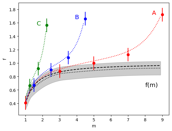
The data are shown in color, with dotted lines showing
the fit results for each set. The fit is
excellent overall. Even at m=9, where the
data pull away, the fit gives 10% accuracy.
These data are artificially generated so we
know what the real f(m) function is.
It is plotted in the figure as a black
dashed line. The fit result for f(m)
agrees well with the exact result for all m.