Case Study: Numerical Analysis inside a Fit
This case study shows how to fit a differential equation,
using gvar.ode, and how to deal with uncertainty in
the independent variable of a fit (that is, the x in
a y versus x fit).
The Problem
A pendulum is released at time 0 from angle 1.571(50) (radians). It’s angular position is measured at intervals of approximately a tenth of second:
t[i]       theta(t[i])
----------------------
0.0          1.571(50)
0.10(1)      1.477(79)
0.20(1)      0.791(79)
0.30(1)     -0.046(79)
0.40(1)     -0.852(79)
0.50(1)     -1.523(79)
0.60(1)     -1.647(79)
0.70(1)     -1.216(79)
0.80(1)     -0.810(79)
0.90(1)      0.185(79)
1.00(1)      0.832(79)
Function theta(t) satisfies a differential equation:
d/dt d/dt theta(t) = -(g/l) sin(theta(t))
where g is the acceleration due to gravity and l is
the pendulum’s length. The challenge is to use the data to improve
our very approximate a priori estimate 40±20 for g/l.
Pendulum Dynamics
We start by designing a data type that solves the differential
equation for theta(t):
import numpy as np
import gvar as gv

class Pendulum(object):
    """ Integrator for pendulum motion.

    Input parameters are:
        g/l .... where g is acceleration due to gravity and l the length
        tol .... precision of numerical integration of ODE
    """
    def __init__(self, g_l, tol=1e-4):
        self.g_l = g_l
        self.odeint = gv.ode.Integrator(deriv=self.deriv, tol=tol)

    def __call__(self, theta0, t_array):
        """ Calculate pendulum angle theta for every t in t_array.

        Assumes that the pendulum is released at time t=0
        from angle theta0 with no initial velocity. Returns
        an array containing theta(t) for every t in t_array.
        """
        # initial values
        t0 = 0
        y0 = [theta0, 0.0]              # theta and dtheta/dt

        # solution  (keep only theta; discard dtheta/dt)
        y = self.odeint.solution(t0, y0)
        return [y(t)[0] for t in t_array]

    def deriv(self, t, y, data=None):
        " Calculate [dtheta/dt, d2theta/dt2] from [theta, dtheta/dt]."
        theta, dtheta_dt = y
        return np.array([dtheta_dt, - self.g_l * gv.sin(theta)])
A Pendulum object is initialized with a value for g/l and a tolerance
for the differential-equation integrator, gvar.ode.Integrator.
Evaluating the object for a given value of theta(0) and t then
calculates theta(t); t is an array. We use gvar.ode here,
rather than some other integrator, because it works with gvar.GVars,
allowing errors to propagate through the integration.
Two Types of Input Data
There are two ways to include data in a fit: either as
regular data, or as fit parameters with priors. In general dependent
variables are treated as regular data, and independent variables with
errors are treated as fit parameters, with priors. Here the dependent
variable is theta(t) and the independent variable is t. The
independent variable has uncertainties, so we treat the individual
values as fit parameters whose priors equal the initial values t[i].
The value of theta(t=0) is also independent data, and so becomes
a fit parameter since it is uncertain. Our fit code therefore
is:
from __future__ import print_function   # makes this work for python2 and 3

import collections
import numpy as np
import gvar as gv
import lsqfit

def main():
    # pendulum data exhibits experimental error in theta and t
    t = gv.gvar([
        '0.10(1)', '0.20(1)', '0.30(1)', '0.40(1)',  '0.50(1)',
        '0.60(1)',  '0.70(1)',  '0.80(1)',  '0.90(1)', '1.00(1)'
        ])
    theta = gv.gvar([
        '1.477(79)', '0.791(79)', '-0.046(79)', '-0.852(79)',
        '-1.523(79)', '-1.647(79)', '-1.216(79)', '-0.810(79)',
        '0.185(79)', '0.832(79)'
        ])

    # priors for all fit parameters: g/l, theta(0), and t[i]
    prior = collections.OrderedDict()
    prior['g/l'] = gv.gvar('40(20)')
    prior['theta(0)'] = gv.gvar('1.571(50)')
    prior['t'] = t

    # fit function: use class Pendulum object to integrate pendulum motion
    def fitfcn(p, t=None):
        if t is None:
            t = p['t']
        pendulum = Pendulum(p['g/l'])
        return pendulum(p['theta(0)'], t)

    # do the fit and print results
    fit = lsqfit.nonlinear_fit(data=theta, prior=prior, fcn=fitfcn)
    print(fit.format(maxline=True))
The prior is a dictionary containing a priori estimates for every fit
parameter. The fit parameters are varied to give the best fit
to both the data and the priors. The fit function uses a Pendulum object
to integrate the differential equation for theta(t), generating values
for each value of t[i] given a value for theta(0).
The function returns an array that has the same shape as array theta.
The fit is excellent with a chi**2 per degree of freedom of 0.7:
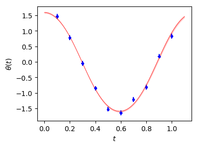
The red band in the figure shows the best fit to the data, with the error bars on the fit. The output from this fit is:
Least Square Fit:
  chi2/dof [dof] = 0.7 [10]    Q = 0.73    logGBF = 6.359

Parameters:
            g/l    39.82 (87)     [    40 (20) ]
       theta(0)    1.595 (32)     [ 1.571 (50) ]
            t 0   0.0960 (91)     [ 0.100 (10) ]
              1   0.2014 (74)     [ 0.200 (10) ]
              2   0.3003 (67)     [ 0.300 (10) ]
              3   0.3982 (76)     [ 0.400 (10) ]
              4   0.5043 (93)     [ 0.500 (10) ]
              5    0.600 (10)     [ 0.600 (10) ]
              6   0.7079 (89)     [ 0.700 (10) ]
              7   0.7958 (79)     [ 0.800 (10) ]
              8   0.9039 (78)     [ 0.900 (10) ]
              9   0.9929 (83)     [ 1.000 (10) ]

Fit:
      key         y[key]      f(p)[key]
---------------------------------------
        0     1.477 (79)     1.412 (42)
        1     0.791 (79)     0.802 (56)
        2    -0.046 (79)    -0.044 (60)
        3    -0.852 (79)    -0.867 (56)
        4    -1.523 (79)    -1.446 (42)
        5    -1.647 (79)    -1.594 (32)
        6    -1.216 (79)    -1.323 (49)  *
        7    -0.810 (79)    -0.776 (61)
        8     0.185 (79)     0.158 (66)
        9     0.832 (79)     0.894 (63)

Settings:
  svdcut/n = 1e-12/0    tol = (1e-08*,1e-10,1e-10)    (itns/time = 7/0.1)
The final result for g/l is 39.8(9), which is accurate to about 2%.
Note that the fit generates (slightly) improved estimates for several of
the t values and for theta(0).