Case Study: Simple Extrapolation
In this case study, we examine a simple extrapolation problem. We show first how not to solve this problem. A better solution follows, together with a discussion of priors and Bayes factors. Finally a very simple, alternative solution, using marginalization, is described.
The Problem
Consider a problem where we have five pieces of uncorrelated data for a
function y(x):
x[i]       y(x[i])
----------------------
0.1        0.5351 (54)
0.3        0.6762 (67)
0.5        0.9227 (91)
0.7        1.3803(131)
0.95       4.0145(399)
We know that y(x) has a Taylor expansion in x:
y(x) = sum_n=0..inf p[n] x**n
The challenge is to extract a reliable estimate for y(0)=p[0] from the
data — that is, the challenge is to fit the data and use
the fit to extrapolate the data to x=0.
A Bad Solution
One approach that is certainly wrong is to fit the data with
a power series expansion for
y(x) that is truncated after five terms (n<=4) —
there are only five pieces of data and such a fit would have five
parameters.
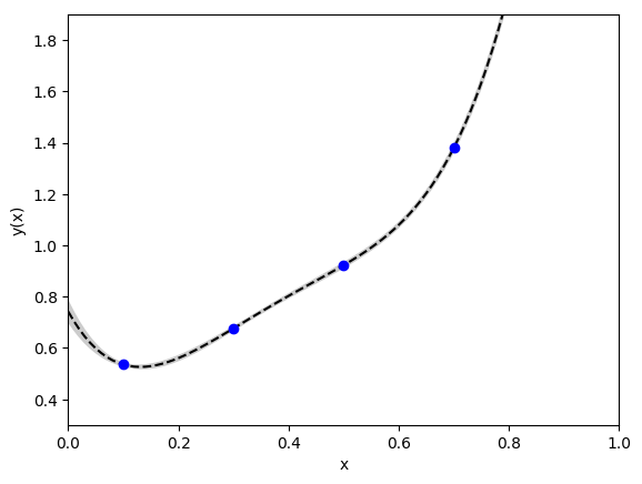
This approach gives the following fit, where the gray band shows the 1-sigma
uncertainty in the fit function evaluated with the best-fit parameters:
This fit was generated using the following code:
import numpy as np
import gvar as gv
import lsqfit

# fit data
y = gv.gvar([
   '0.5351(54)', '0.6762(67)', '0.9227(91)', '1.3803(131)', '4.0145(399)'
   ])
x = np.array([0.1, 0.3, 0.5, 0.7, 0.95])

# fit function
def f(x, p):
   return sum(pn * x ** n for n, pn in enumerate(p))

p0 = np.ones(5.)              # starting value for chi**2 minimization
fit = lsqfit.nonlinear_fit(data=(x, y), p0=p0, fcn=f)
print(fit.format(maxline=True))
Note that here the function gv.gvar converts the strings
'0.5351(54)', etc. into gvar.GVars. Running the code gives the
following output:
Least Square Fit (no prior):
  chi2/dof [dof] = 4.5e-24 [0]    Q = 0    logGBF = None

Parameters:
              0    0.742 (39)     [   1 +- inf ]
              1    -3.86 (59)     [   1 +- inf ]
              2    21.5 (2.4)     [   1 +- inf ]
              3   -39.1 (3.7)     [   1 +- inf ]
              4    25.8 (1.9)     [   1 +- inf ]

Fit:
     x[k]           y[k]      f(x[k],p)
---------------------------------------
      0.1    0.5351 (54)    0.5351 (54)
      0.3    0.6762 (67)    0.6762 (67)
      0.5    0.9227 (91)    0.9227 (91)
      0.7     1.380 (13)     1.380 (13)
     0.95     4.014 (40)     4.014 (40)

Settings:
  svdcut/n = 1e-12/0    tol = (1e-08*,1e-10,1e-10)    (itns/time = 11/0.0)
This is a “perfect” fit in that the fit function agrees exactly with
the data; the chi**2 for the fit is zero. The 5-parameter fit
gives a fairly precise answer for p[0]
(0.74(4)), but the curve looks oddly stiff. Also some of the
best-fit values for the coefficients are quite
large (e.g., p[3]= -39(4)), perhaps unreasonably large.
A Better Solution — Priors
The problem with a 5-parameter fit is that there is no reason to neglect
terms in the expansion of y(x) with n>4. Whether or not
extra terms are important depends entirely on how large we
expect the coefficients p[n] for n>4 to be. The extrapolation
problem is impossible without some idea of the size of these
parameters; we need extra information.
In this case that extra information is obviously connected to questions
of convergence of the Taylor expansion we are using to model y(x).
Let’s assume we know, from previous work, that the p[n] are of
order one. Then we would need to keep at least 91 terms in the
Taylor expansion if we wanted the terms we dropped to be small compared
with the 1% data errors at x=0.95. So a possible fitting function
would be:
y(x; N) = sum_n=0..N p[n] x**n
with N=90.
Fitting a 91-parameter formula to five pieces of data is also impossible. Here, however, we have extra (prior) information: each coefficient is order one, which we make specific by saying that they equal 0±1. We include these a priori estimates for the parameters as extra data that must be fit, together with our original data. So we are actually fitting 91+5 pieces of data with 91 parameters.
The prior information is introduced into the fit as a prior:
import numpy as np
import gvar as gv
import lsqfit

# fit data
y = gv.gvar([
   '0.5351(54)', '0.6762(67)', '0.9227(91)', '1.3803(131)', '4.0145(399)'
   ])
x = np.array([0.1, 0.3, 0.5, 0.7, 0.95])

# fit function
def f(x, p):
   return sum(pn * x ** n for n, pn in enumerate(p))

# 91-parameter prior for the fit
prior = gv.gvar(91 * ['0(1)'])

fit = lsqfit.nonlinear_fit(data=(x, y), prior=prior, fcn=f)
print(fit.format(maxline=True))
Note that a starting value p0 is not needed when a prior is specified.
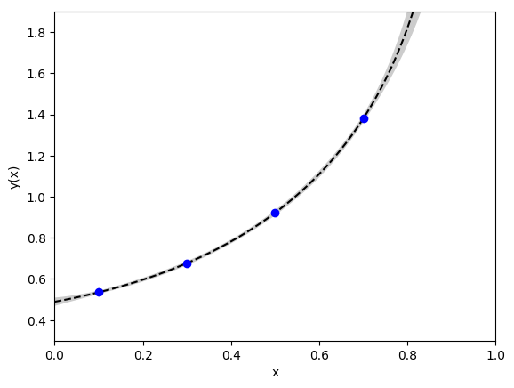
This code also gives an excellent fit, with a chi**2 per degree of
freedom of 0.35 (note that the data point at x=0.95 is off the chart,
but agrees with the fit to within its 1% errors):
The fit code output is:
Least Square Fit:
  chi2/dof [dof] = 0.35 [5]    Q = 0.88    logGBF = -0.45508

Parameters:
              0      0.489 (17)      [  0.0 (1.0) ]
              1       0.40 (20)      [  0.0 (1.0) ]
              2       0.60 (64)      [  0.0 (1.0) ]
              3       0.44 (80)      [  0.0 (1.0) ]
              4       0.28 (87)      [  0.0 (1.0) ]
              5       0.19 (87)      [  0.0 (1.0) ]
              6       0.16 (90)      [  0.0 (1.0) ]
              7       0.16 (93)      [  0.0 (1.0) ]
              8       0.17 (95)      [  0.0 (1.0) ]
              9       0.18 (96)      [  0.0 (1.0) ]
             10       0.19 (97)      [  0.0 (1.0) ]
             11       0.19 (97)      [  0.0 (1.0) ]
             12       0.19 (97)      [  0.0 (1.0) ]
             13       0.19 (97)      [  0.0 (1.0) ]
             14       0.18 (97)      [  0.0 (1.0) ]
             15       0.18 (97)      [  0.0 (1.0) ]
             16       0.17 (97)      [  0.0 (1.0) ]
             17       0.16 (98)      [  0.0 (1.0) ]
             18       0.16 (98)      [  0.0 (1.0) ]
             19       0.15 (98)      [  0.0 (1.0) ]
             20       0.14 (98)      [  0.0 (1.0) ]
             21       0.14 (98)      [  0.0 (1.0) ]
             22       0.13 (98)      [  0.0 (1.0) ]
             23       0.12 (99)      [  0.0 (1.0) ]
             24       0.12 (99)      [  0.0 (1.0) ]
             25       0.11 (99)      [  0.0 (1.0) ]
             26       0.11 (99)      [  0.0 (1.0) ]
             27       0.10 (99)      [  0.0 (1.0) ]
             28       0.10 (99)      [  0.0 (1.0) ]
             29       0.09 (99)      [  0.0 (1.0) ]
             30       0.09 (99)      [  0.0 (1.0) ]
             31       0.08 (99)      [  0.0 (1.0) ]
             32       0.08 (99)      [  0.0 (1.0) ]
             33       0.07 (99)      [  0.0 (1.0) ]
             34     0.07 (1.00)      [  0.0 (1.0) ]
             35     0.07 (1.00)      [  0.0 (1.0) ]
             36     0.06 (1.00)      [  0.0 (1.0) ]
             37     0.06 (1.00)      [  0.0 (1.0) ]
             38     0.06 (1.00)      [  0.0 (1.0) ]
             39     0.06 (1.00)      [  0.0 (1.0) ]
             40     0.05 (1.00)      [  0.0 (1.0) ]
             41     0.05 (1.00)      [  0.0 (1.0) ]
             42     0.05 (1.00)      [  0.0 (1.0) ]
             43     0.04 (1.00)      [  0.0 (1.0) ]
             44     0.04 (1.00)      [  0.0 (1.0) ]
             45     0.04 (1.00)      [  0.0 (1.0) ]
             46     0.04 (1.00)      [  0.0 (1.0) ]
             47     0.04 (1.00)      [  0.0 (1.0) ]
             48     0.03 (1.00)      [  0.0 (1.0) ]
             49     0.03 (1.00)      [  0.0 (1.0) ]
             50     0.03 (1.00)      [  0.0 (1.0) ]
             51     0.03 (1.00)      [  0.0 (1.0) ]
             52     0.03 (1.00)      [  0.0 (1.0) ]
             53     0.03 (1.00)      [  0.0 (1.0) ]
             54     0.03 (1.00)      [  0.0 (1.0) ]
             55     0.02 (1.00)      [  0.0 (1.0) ]
             56     0.02 (1.00)      [  0.0 (1.0) ]
             57     0.02 (1.00)      [  0.0 (1.0) ]
             58     0.02 (1.00)      [  0.0 (1.0) ]
             59     0.02 (1.00)      [  0.0 (1.0) ]
             60     0.02 (1.00)      [  0.0 (1.0) ]
             61     0.02 (1.00)      [  0.0 (1.0) ]
             62     0.02 (1.00)      [  0.0 (1.0) ]
             63     0.02 (1.00)      [  0.0 (1.0) ]
             64     0.02 (1.00)      [  0.0 (1.0) ]
             65     0.01 (1.00)      [  0.0 (1.0) ]
             66     0.01 (1.00)      [  0.0 (1.0) ]
             67     0.01 (1.00)      [  0.0 (1.0) ]
             68     0.01 (1.00)      [  0.0 (1.0) ]
             69     0.01 (1.00)      [  0.0 (1.0) ]
             70     0.01 (1.00)      [  0.0 (1.0) ]
             71     0.01 (1.00)      [  0.0 (1.0) ]
             72     0.01 (1.00)      [  0.0 (1.0) ]
             73     0.01 (1.00)      [  0.0 (1.0) ]
             74   0.009 (1.000)      [  0.0 (1.0) ]
             75   0.009 (1.000)      [  0.0 (1.0) ]
             76   0.008 (1.000)      [  0.0 (1.0) ]
             77   0.008 (1.000)      [  0.0 (1.0) ]
             78   0.007 (1.000)      [  0.0 (1.0) ]
             79   0.007 (1.000)      [  0.0 (1.0) ]
             80   0.007 (1.000)      [  0.0 (1.0) ]
             81   0.006 (1.000)      [  0.0 (1.0) ]
             82   0.006 (1.000)      [  0.0 (1.0) ]
             83   0.006 (1.000)      [  0.0 (1.0) ]
             84   0.005 (1.000)      [  0.0 (1.0) ]
             85   0.005 (1.000)      [  0.0 (1.0) ]
             86   0.005 (1.000)      [  0.0 (1.0) ]
             87   0.005 (1.000)      [  0.0 (1.0) ]
             88   0.004 (1.000)      [  0.0 (1.0) ]
             89   0.004 (1.000)      [  0.0 (1.0) ]
             90   0.004 (1.000)      [  0.0 (1.0) ]

Fit:
     x[k]           y[k]      f(x[k],p)
---------------------------------------
      0.1    0.5351 (54)    0.5349 (54)
      0.3    0.6762 (67)    0.6768 (65)
      0.5    0.9227 (91)    0.9219 (87)
      0.7     1.380 (13)     1.381 (13)
     0.95     4.014 (40)     4.014 (40)

Settings:
  svdcut/n = 1e-12/0    tol = (1e-08*,1e-10,1e-10)    (itns/time = 8/0.1)
This is a much more plausible fit than than the 5-parameter fit, and gives an
extrapolated value of p[0]=0.489(17). The original data points were
created using a Taylor expansion with random coefficients, but
with p[0] set equal to 0.5. So this fit to the five data points (plus
91 a priori values for the p[n] with n<91) gives the correct
result. Increasing the number of terms further would have no effect since the
last terms added are having no impact, and so end up equal to the prior value
— the fit data are not sufficiently precise to add new information about
these parameters.
Bayes Factors
We can test our priors for this fit by re-doing the fit with broader and
narrower priors. Setting prior = gv.gvar(91 * ['0(3)']) gives an excellent
fit,
Least Square Fit:
  chi2/dof [dof] = 0.039 [5]    Q = 1    logGBF = -5.0993

Parameters:
              0      0.490 (33)      [  0.0 (3.0) ]
              1       0.38 (48)      [  0.0 (3.0) ]
              2       0.6 (1.8)      [  0.0 (3.0) ]
              3       0.5 (2.4)      [  0.0 (3.0) ]
              4       0.3 (2.6)      [  0.0 (3.0) ]
              5       0.2 (2.6)      [  0.0 (3.0) ]
              6       0.1 (2.7)      [  0.0 (3.0) ]
              7       0.1 (2.8)      [  0.0 (3.0) ]
              8       0.2 (2.8)      [  0.0 (3.0) ]
              9       0.2 (2.9)      [  0.0 (3.0) ]
             10       0.2 (2.9)      [  0.0 (3.0) ]
             11       0.2 (2.9)      [  0.0 (3.0) ]
             12       0.2 (2.9)      [  0.0 (3.0) ]
             13       0.2 (2.9)      [  0.0 (3.0) ]
             14       0.2 (2.9)      [  0.0 (3.0) ]
             15       0.2 (2.9)      [  0.0 (3.0) ]
             16       0.2 (2.9)      [  0.0 (3.0) ]
             17       0.2 (2.9)      [  0.0 (3.0) ]
             18       0.2 (2.9)      [  0.0 (3.0) ]
             19       0.2 (2.9)      [  0.0 (3.0) ]
             20       0.1 (2.9)      [  0.0 (3.0) ]
             21       0.1 (2.9)      [  0.0 (3.0) ]
             22       0.1 (2.9)      [  0.0 (3.0) ]
             23       0.1 (3.0)      [  0.0 (3.0) ]
             24       0.1 (3.0)      [  0.0 (3.0) ]
             25       0.1 (3.0)      [  0.0 (3.0) ]
             26       0.1 (3.0)      [  0.0 (3.0) ]
             27       0.1 (3.0)      [  0.0 (3.0) ]
             28       0.1 (3.0)      [  0.0 (3.0) ]
             29       0.1 (3.0)      [  0.0 (3.0) ]
             30     0.09 (2.98)      [  0.0 (3.0) ]
             31     0.09 (2.98)      [  0.0 (3.0) ]
             32     0.08 (2.98)      [  0.0 (3.0) ]
             33     0.08 (2.98)      [  0.0 (3.0) ]
             34     0.07 (2.99)      [  0.0 (3.0) ]
             35     0.07 (2.99)      [  0.0 (3.0) ]
             36     0.07 (2.99)      [  0.0 (3.0) ]
             37     0.06 (2.99)      [  0.0 (3.0) ]
             38     0.06 (2.99)      [  0.0 (3.0) ]
             39     0.06 (2.99)      [  0.0 (3.0) ]
             40     0.05 (2.99)      [  0.0 (3.0) ]
             41     0.05 (2.99)      [  0.0 (3.0) ]
             42     0.05 (2.99)      [  0.0 (3.0) ]
             43     0.05 (2.99)      [  0.0 (3.0) ]
             44     0.04 (2.99)      [  0.0 (3.0) ]
             45     0.04 (3.00)      [  0.0 (3.0) ]
             46     0.04 (3.00)      [  0.0 (3.0) ]
             47     0.04 (3.00)      [  0.0 (3.0) ]
             48     0.04 (3.00)      [  0.0 (3.0) ]
             49     0.03 (3.00)      [  0.0 (3.0) ]
             50     0.03 (3.00)      [  0.0 (3.0) ]
             51     0.03 (3.00)      [  0.0 (3.0) ]
             52     0.03 (3.00)      [  0.0 (3.0) ]
             53     0.03 (3.00)      [  0.0 (3.0) ]
             54     0.03 (3.00)      [  0.0 (3.0) ]
             55     0.03 (3.00)      [  0.0 (3.0) ]
             56     0.02 (3.00)      [  0.0 (3.0) ]
             57     0.02 (3.00)      [  0.0 (3.0) ]
             58     0.02 (3.00)      [  0.0 (3.0) ]
             59     0.02 (3.00)      [  0.0 (3.0) ]
             60     0.02 (3.00)      [  0.0 (3.0) ]
             61     0.02 (3.00)      [  0.0 (3.0) ]
             62     0.02 (3.00)      [  0.0 (3.0) ]
             63     0.02 (3.00)      [  0.0 (3.0) ]
             64     0.02 (3.00)      [  0.0 (3.0) ]
             65     0.02 (3.00)      [  0.0 (3.0) ]
             66     0.01 (3.00)      [  0.0 (3.0) ]
             67     0.01 (3.00)      [  0.0 (3.0) ]
             68     0.01 (3.00)      [  0.0 (3.0) ]
             69     0.01 (3.00)      [  0.0 (3.0) ]
             70     0.01 (3.00)      [  0.0 (3.0) ]
             71     0.01 (3.00)      [  0.0 (3.0) ]
             72     0.01 (3.00)      [  0.0 (3.0) ]
             73     0.01 (3.00)      [  0.0 (3.0) ]
             74   0.009 (3.000)      [  0.0 (3.0) ]
             75   0.009 (3.000)      [  0.0 (3.0) ]
             76   0.009 (3.000)      [  0.0 (3.0) ]
             77   0.008 (3.000)      [  0.0 (3.0) ]
             78   0.008 (3.000)      [  0.0 (3.0) ]
             79   0.007 (3.000)      [  0.0 (3.0) ]
             80   0.007 (3.000)      [  0.0 (3.0) ]
             81   0.007 (3.000)      [  0.0 (3.0) ]
             82   0.006 (3.000)      [  0.0 (3.0) ]
             83   0.006 (3.000)      [  0.0 (3.0) ]
             84   0.006 (3.000)      [  0.0 (3.0) ]
             85   0.005 (3.000)      [  0.0 (3.0) ]
             86   0.005 (3.000)      [  0.0 (3.0) ]
             87   0.005 (3.000)      [  0.0 (3.0) ]
             88   0.005 (3.000)      [  0.0 (3.0) ]
             89   0.004 (3.000)      [  0.0 (3.0) ]
             90   0.004 (3.000)      [  0.0 (3.0) ]

Fit:
     x[k]           y[k]      f(x[k],p)
---------------------------------------
      0.1    0.5351 (54)    0.5351 (54)
      0.3    0.6762 (67)    0.6763 (67)
      0.5    0.9227 (91)    0.9226 (91)
      0.7     1.380 (13)     1.380 (13)
     0.95     4.014 (40)     4.014 (40)

Settings:
  svdcut/n = 1e-12/0    tol = (1e-08,1e-10*,1e-10)    (itns/time = 9/0.1)
but with a very small chi2/dof and somewhat larger errors on the best-fit
estimates for the parameters. The logarithm of the (Gaussian) Bayes Factor,
logGBF, can be used to compare fits with different priors. It is the
logarithm of the probability that our data would come from parameters
generated at random using the prior. The exponential of logGBF is
more than 100 times larger with the original priors of 0(1) than with
priors of 0(3). This says that our data is more than 100 times more
likely to come from a world with parameters of order one than from one with
parameters of order three. Put another way it says that
the size of the fluctuations in the data
are more consistent with coefficients of order one than with coefficients of
order three — in the latter case, there would have been larger
fluctuations in the data than are actually seen.
The logGBF values argue for the original prior.
Narrower priors, prior = gv.gvar(91 * ['0.0(3)']), give a poor fit,
and also a less optimal logGBF:
Least Square Fit:
  chi2/dof [dof] = 3.7 [5]    Q = 0.0024    logGBF = -3.3058

Parameters:
              0    0.484 (11)     [  0.00 (30) ]  *
              1    0.454 (98)     [  0.00 (30) ]  *
              2     0.50 (23)     [  0.00 (30) ]  *
              3     0.40 (25)     [  0.00 (30) ]  *
              4     0.31 (26)     [  0.00 (30) ]  *
              5     0.26 (27)     [  0.00 (30) ]
              6     0.23 (28)     [  0.00 (30) ]
              7     0.21 (29)     [  0.00 (30) ]
              8     0.21 (29)     [  0.00 (30) ]
              9     0.20 (29)     [  0.00 (30) ]
             10     0.19 (29)     [  0.00 (30) ]
             11     0.19 (29)     [  0.00 (30) ]
             12     0.18 (29)     [  0.00 (30) ]
             13     0.17 (29)     [  0.00 (30) ]
             14     0.17 (29)     [  0.00 (30) ]
             15     0.16 (29)     [  0.00 (30) ]
             16     0.15 (29)     [  0.00 (30) ]
             17     0.15 (29)     [  0.00 (30) ]
             18     0.14 (29)     [  0.00 (30) ]
             19     0.13 (29)     [  0.00 (30) ]
             20     0.13 (29)     [  0.00 (30) ]
             21     0.12 (30)     [  0.00 (30) ]
             22     0.11 (30)     [  0.00 (30) ]
             23     0.11 (30)     [  0.00 (30) ]
             24     0.10 (30)     [  0.00 (30) ]
             25     0.10 (30)     [  0.00 (30) ]
             26     0.09 (30)     [  0.00 (30) ]
             27     0.09 (30)     [  0.00 (30) ]
             28     0.08 (30)     [  0.00 (30) ]
             29     0.08 (30)     [  0.00 (30) ]
             30     0.08 (30)     [  0.00 (30) ]
             31     0.07 (30)     [  0.00 (30) ]
             32     0.07 (30)     [  0.00 (30) ]
             33     0.07 (30)     [  0.00 (30) ]
             34     0.06 (30)     [  0.00 (30) ]
             35     0.06 (30)     [  0.00 (30) ]
             36     0.06 (30)     [  0.00 (30) ]
             37     0.05 (30)     [  0.00 (30) ]
             38     0.05 (30)     [  0.00 (30) ]
             39     0.05 (30)     [  0.00 (30) ]
             40     0.05 (30)     [  0.00 (30) ]
             41     0.04 (30)     [  0.00 (30) ]
             42     0.04 (30)     [  0.00 (30) ]
             43     0.04 (30)     [  0.00 (30) ]
             44     0.04 (30)     [  0.00 (30) ]
             45     0.04 (30)     [  0.00 (30) ]
             46     0.03 (30)     [  0.00 (30) ]
             47     0.03 (30)     [  0.00 (30) ]
             48     0.03 (30)     [  0.00 (30) ]
             49     0.03 (30)     [  0.00 (30) ]
             50     0.03 (30)     [  0.00 (30) ]
             51     0.03 (30)     [  0.00 (30) ]
             52     0.02 (30)     [  0.00 (30) ]
             53     0.02 (30)     [  0.00 (30) ]
             54     0.02 (30)     [  0.00 (30) ]
             55     0.02 (30)     [  0.00 (30) ]
             56     0.02 (30)     [  0.00 (30) ]
             57     0.02 (30)     [  0.00 (30) ]
             58     0.02 (30)     [  0.00 (30) ]
             59     0.02 (30)     [  0.00 (30) ]
             60     0.02 (30)     [  0.00 (30) ]
             61     0.02 (30)     [  0.00 (30) ]
             62     0.01 (30)     [  0.00 (30) ]
             63     0.01 (30)     [  0.00 (30) ]
             64     0.01 (30)     [  0.00 (30) ]
             65     0.01 (30)     [  0.00 (30) ]
             66     0.01 (30)     [  0.00 (30) ]
             67     0.01 (30)     [  0.00 (30) ]
             68     0.01 (30)     [  0.00 (30) ]
             69     0.01 (30)     [  0.00 (30) ]
             70     0.01 (30)     [  0.00 (30) ]
             71   0.009 (300)     [  0.00 (30) ]
             72   0.009 (300)     [  0.00 (30) ]
             73   0.008 (300)     [  0.00 (30) ]
             74   0.008 (300)     [  0.00 (30) ]
             75   0.008 (300)     [  0.00 (30) ]
             76   0.007 (300)     [  0.00 (30) ]
             77   0.007 (300)     [  0.00 (30) ]
             78   0.006 (300)     [  0.00 (30) ]
             79   0.006 (300)     [  0.00 (30) ]
             80   0.006 (300)     [  0.00 (30) ]
             81   0.006 (300)     [  0.00 (30) ]
             82   0.005 (300)     [  0.00 (30) ]
             83   0.005 (300)     [  0.00 (30) ]
             84   0.005 (300)     [  0.00 (30) ]
             85   0.005 (300)     [  0.00 (30) ]
             86   0.004 (300)     [  0.00 (30) ]
             87   0.004 (300)     [  0.00 (30) ]
             88   0.004 (300)     [  0.00 (30) ]
             89   0.004 (300)     [  0.00 (30) ]
             90   0.003 (300)     [  0.00 (30) ]

Fit:
     x[k]           y[k]      f(x[k],p)
---------------------------------------
      0.1    0.5351 (54)    0.5344 (53)
      0.3    0.6762 (67)    0.6787 (56)
      0.5    0.9227 (91)    0.9191 (75)
      0.7     1.380 (13)     1.382 (13)
     0.95     4.014 (40)     4.008 (40)

Settings:
  svdcut/n = 1e-12/0    tol = (1e-08*,1e-10,1e-10)    (itns/time = 6/0.1)
Setting prior = gv.gvar(91 * ['0(20)']) gives very wide priors and
a rather strange looking fit:
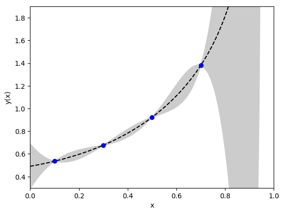
Here fit errors are comparable to the data errors at the data points, as you
would expect, but balloon up in between. This is an example of
over-fitting: the data and priors are not sufficiently accurate to fit the
number of parameters used. Specifically the priors are too broad.
Again the Bayes Factor signals the problem: logGBF = -14.479 here, which
means that our data are roughly a million times (=exp(14)) more
likely to to come from a world with coefficients of order one than
from one with coefficients of order twenty. That is, the broad priors suggest
much larger
variations between the leading parameters than is indicated by the data —
again, the
data are unnaturally regular in a world described by the very broad prior.
Absent useful a priori information about the parameters, we can sometimes use the
data to suggest a plausible width for a set of priors. We do this by setting
the width equal to the value
that maximizes logGBF. This approach suggests priors of 0.0(6) for
the fit above, which gives results very similar to the fit
with priors of 0(1). See Tuning Priors with the Empirical Bayes Criterion for more details.
The priors are responsible for about half of the final error in our best
estimate of p[0] (with priors of 0(1)); the rest comes from the
uncertainty in the data. This can be established by creating an error budget
using the code
inputs = dict(prior=prior, y=y)
outputs = dict(p0=fit.p[0])
print(gv.fmt_errorbudget(inputs=inputs, outputs=outputs))
which prints the following table:
Partial % Errors:
                  p0
--------------------
        y:      2.67
    prior:      2.23
--------------------
    total:      3.48
The table shows that the final 3.5% error comes from a 2.7% error due
to uncertainties in y and a 2.2% error from uncertainties in the
prior (added in quadrature).
Another Solution — Marginalization
There is a second, equivalent way of fitting this data that illustrates the
idea of marginalization. We really only care about parameter p[0] in
our fit. This suggests that we remove n>0 terms from the data before
we do the fit:
ymod[i] = y[i] - sum_n=1...inf prior[n] * x[i] ** n
Before the fit, our best estimate for the parameters is from the priors. We
use these to create an estimate for the correction to each data point
coming from n>0 terms in y(x). This new data, ymod[i],
should be fit with
a new fitting function, ymod(x) = p[0] — that is, it should be fit
to a constant, independent of x[i]. The last three lines of the code
above are easily modified to implement this idea:
import numpy as np
import gvar as gv
import lsqfit

# fit data
y = gv.gvar([
   '0.5351(54)', '0.6762(67)', '0.9227(91)', '1.3803(131)', '4.0145(399)'
   ])
x = np.array([0.1, 0.3, 0.5, 0.7, 0.95])

# fit function
def f(x, p):
   return sum(pn * x ** n for n, pn in enumerate(p))

# prior for the fit
prior = gv.gvar(91 * ['0(1)'])

# marginalize all but one parameter (p[0])
priormod = prior[:1]                       # restrict fit to p[0]
ymod = y - (f(x, prior) - f(x, priormod))  # correct y

fit = lsqfit.nonlinear_fit(data=(x, ymod), prior=priormod, fcn=f)
print(fit.format(maxline=True))
Running this code give:
Least Square Fit:
  chi2/dof [dof] = 0.35 [5]    Q = 0.88    logGBF = -0.45508

Parameters:
              0   0.489 (17)     [  0.0 (1.0) ]

Fit:
     x[k]         y[k]     f(x[k],p)
------------------------------------
      0.1    0.54 (10)    0.489 (17)
      0.3    0.68 (31)    0.489 (17)
      0.5    0.92 (58)    0.489 (17)
      0.7    1.38 (98)    0.489 (17)
     0.95    4.0 (3.0)    0.489 (17)  *

Settings:
  svdcut/n = 1e-12/0    tol = (1e-08*,1e-10,1e-10)    (itns/time = 4/0.0)
Remarkably this one-parameter fit gives results for p[0]
that are identical (to
machine precision) to our 91-parameter fit above. The 90 parameters for
n>0 are said to have been marginalized in this fit.
Marginalizing a parameter
in this way has no effect if the fit function is linear in that parameter.
Marginalization has almost no effect for nonlinear fits as well,
provided the fit data have small errors (in which case the parameters are
effectively linear). The fit here is:
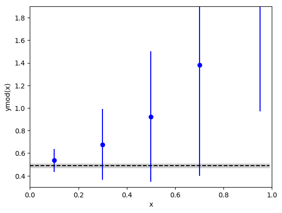
The constant is consistent with all of the data in ymod[i],
even at x[i]=0.95, because ymod[i] has much larger errors for
larger x[i] because of the correction terms.
Fitting to a constant is equivalent to doing a weighted average of the data plus the prior, so our fit can be replaced by an average:
lsqfit.wavg(list(ymod) + list(priormod))
This again gives 0.489(17) for our final result.
Note that the central value for this average is below the central
values for every data point in ymod[i]. This is a consequence of large
positive correlations introduced into ymod when we remove the
n>0 terms. These correlations are captured automatically in our code,
and are essential — removing the correlations between different
ymods results in a final answer, 0.564(97), which has a much
larger error.